Best practices for faster SQL
Learn the best practices when working with a huge amount of data. We recommend that all Tinybird users read this.
When you're trying to process huge amounts of data, there's some best practices to follow. These are hard-learned lessons from years of building realtime systems at huge scale.
The 5 Rules of Fast Queries
We don't want our users to waste any time. So, we have created a cheatsheet of rules you can consult whenever you need help to go fast.
We like to call them The 5 Rules of Fast Queries:
- Rule № 1 ⟶ The best data is the one you don't write.
- Rule № 2 ⟶ The second best data is the one you don't read. (The less data you read, the better.)
- Rule № 3 ⟶ Sequential reads are 100x faster.
- Rule № 4 ⟶ The less data you process (after read), the better.
- Rule № 5 ⟶ Complex operations later in the processing pipeline.
Let's go one by one, analyzing the improvement of the performance after the implementation of each rule. We will use the already-so-well-known NYC Taxi Trip dataset. You can get a sample here and import it directly creating a new Data Source from your dashboard.
Rule 1: The best data is the one you don't write
This rule seems obvious but it's not always followed. There is no reason to save data that you don't need: it will impact the memory needed (and the money!) and the queries will take more time, so it only has disadvantages.
Rule 2: The second best data is the one you don't read
To avoid reading data that you don't need, you should apply filters as soon as possible.
For this example, let's suppose we want a list of the trips whose distance is greater than 10 miles and that took place between '2017-01-31 14:00:00' and '2017-01-31 15:00:00'. Additionally, we want to get those trips ordered by date.
Let's see the difference between applying the filters at the end or at the beginning of the pipe.
First, let's start the first approach by ordering all the data by date:
Once the data is sorted, we filter it:
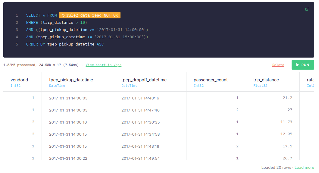
This first approach takes around 30-60 ms, adding the time of both steps.
Pay attention to the statistics in the first step: number of scanned rows (139.26k) and the size of data (10.31MB) vs statistics in the second one: number of scanned rows (24.58k) and the size of data (1.82MB). Why would we scan 139.26k rows in the first place if we just really need to scan 24.58k?
It's important to be aware that these two values directly impact the query execution time and also affect other queries you may be running at the same time. IO bandwidth is also something you need to keep in mind.
Let's see what happens if the filter is applied before the sorting:
As can be seen, if the filter is applied before the sorting, it takes only 1-10 ms. If you take a look at the size of the data read, it's 1.82MB, while the number of rows read is 24.58k. As explained, they are much smaller than the ones in the first step.
This significant difference happens because in the first approach, we are sorting all the data available (even the data that we don't need for our query) while in the second approach, we are sorting just the rows we need.
Filtering is the fastest operation, so always filter first.
Rule 3: Sequential reads are 100x faster
To be able to carry out sequential reads, it's essential to define indexes correctly. These indexes should be defined based on the queries that are going to be performed. (Although these indexes should be defined in the Data Source, we will simulate the case by ordering the data based on the columns.)
For example, if we want to query the data by date, let's compare what happens when the data is sorted by date vs when it's sorted by any other column.
In the first approach, we will sort the data by another column, for instance, ""passenger_count"":
Once we have the data sorted by ""passenger_count"", we filter it by date:
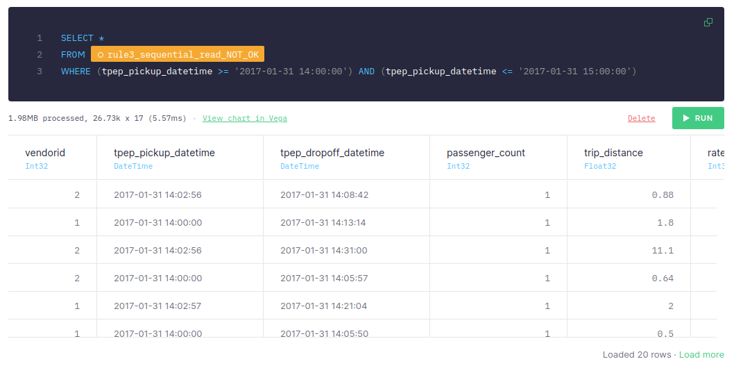
This approach takes around 5-10 ms, the number of scanned rows is 26.73k and the size of data is 1.98MB.
For the second approach, we are sorting the data by date:
Once it's sorted by date, we filter it:
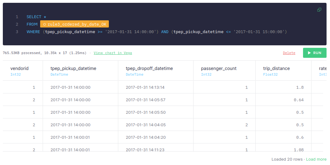
We can see that if the data is sorted by date and the query uses date for filtering, it just takes 1-2 ms, the number of scanned rows is 10.35k and the size of data is 765.53KB. Let's remember that the first approach takes around 5-10 ms, the number of scanned rows is 26.73k and the size of data is 1.98MB.
It's important to highlight that the more data we have, the greater will be the difference between both approaches. When dealing with tons of data, sequential reads can be 100x faster.
Therefore, it's essential to define the indexes taking into account the queries that will be made.
Rule 4: The less data you process (after read), the better
So, if you just need two columns, only retrieve those.
Let's suppose that for our use case, we just need three columns: vendorid, tpep_pickup_datetime and trip_distance.
Let's analyze the difference between retrieving all the columns vs just the ones we need.
When retrieving all the columns, we need around 140-180 ms and the size of data is 718.55MB:
However, when retrieving just the columns we need, it takes around 35-60 ms:
As we mentioned before, you can check how the size of scanned data is much less, now just 155.36MB. With analytical databases, if you do not need to retrieve a column, those files are not read and it is much more efficient.
Therefore, it's strongly recommended to process just the data needed.
Rule 5: Complex operations later in the processing pipeline
Complex operations, such as joins or aggregations, should be performed as late as possible in the processing pipeline. This is because in the first steps you should filter all the data, so the number of rows at the end will be less than at the beginning and, therefore, the cost of executing complex operations will be lower.
So first, let's aggregate the data:
Now, let's apply the filter:
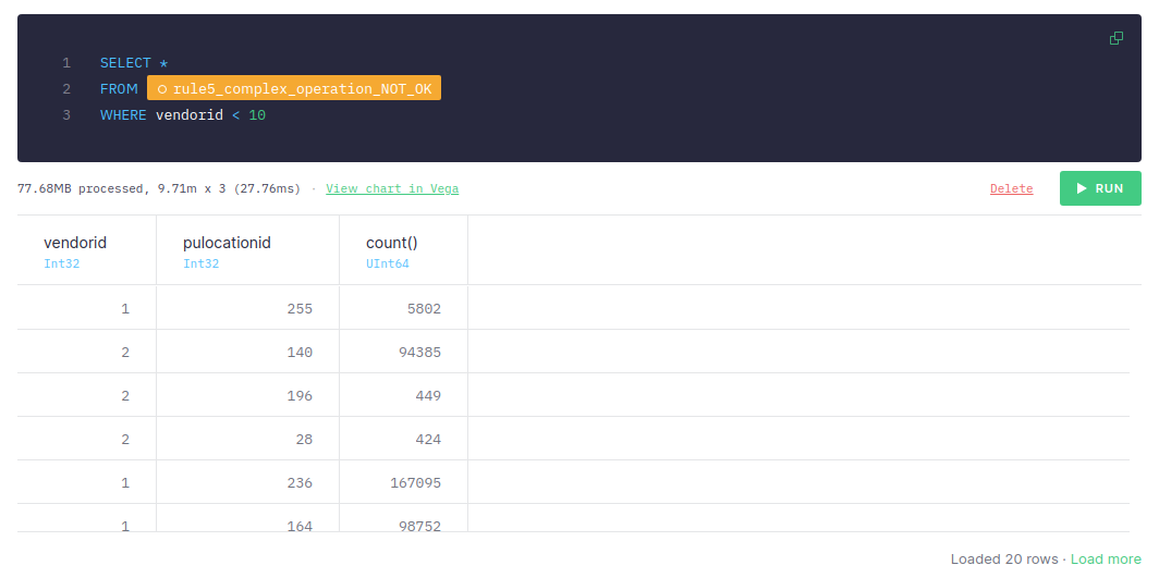
If the filter is applied after aggregating the data, it takes around 50-70 ms to retrieve the data (adding both steps), the number of scanned rows is 9.71m and the size of data is 77.68MB.
Let's see what happens if we filter before aggregating the data:
Doing it this way, it takes only 20-40 ms, although the number of scanned rows and the size of data is the same as in the previous approach.
Therefore, it's recommended to perform complex operations as late as possible in the processing pipeline.
Additional guidance
If that wasn't enough, here's some more general advice:
Avoiding full scans
The less data you read in your queries, the faster they are. There are different strategies you could follow to avoid reading all the data in a data source (doing a full scan) from your queries:
- Always filter first
- Use indices by setting a proper
ENGINE_SORTING_KEYin the Data Source. - The column names present in the
ENGINE_SORTING_KEYshould be the ones you will use for filtering in theWHEREclause. You don't need to sort by all the columns you use for filtering, only the ones to filter first. - The order of the columns in the
ENGINE_SORTING_KEYis important: from left to right ordered by relevance (the more important ones for filtering) and cardinality (less cardinality goes first)
Data Source: data_source_sorted_by_date
SCHEMA >
  `id` Int64,
  `amount` Int64,
  `date` DateTime

ENGINE "MergeTree"
ENGINE_SORTING_KEY "id, date"
BAD: Not filtering by any column present in the ENGINE_SORTING_KEY
SELECT *
FROM data_source_sorted_by_date
WHERE amount > 30
GOOD: Filtering first by columns present in the ENGINE_SORTING_KEY
SELECT *
FROM data_source_sorted_by_date
WHERE
  id = 135246 AND
  date > now() - INTERVAL 3 DAY AND
  amount > 30
Avoiding big joins
When doing a JOIN, the data in the right Data Source is loaded in memory to perform the JOIN. Therefore, it's recommended to avoid joining big Data Sources by filtering the data in the right Data Source:
JOINs over tables of more than 1M rows might lead to MEMORY_LIMIT errors when used in Materialized Views, affecting ingestion.
A common pattern to improve JOIN performance is the one below:
BAD: Doing a JOIN with a Data Source with too many rows
SELECT
    left.id AS id,
    left.date AS day,
    right.response_id AS response_id
FROM left_data_source AS left
INNER JOIN big_right_data_source AS right ON left.id = right.id
GOOD: Prefilter the joined Data Source for better performance
SELECT
    left.id AS id,
    left.date AS day,
    right.response_id AS response_id
FROM left_data_source AS left
INNER JOIN (
  SELECT id, response_id
  FROM big_right_data_source
  WHERE id IN (SELECT id FROM left_data_source)
) AS right ON left.id = right.id
Memory limit reached
Sometimes, you reach the memory limit when running a query. This is usually because:
- Lot of columns are used: try to reduce the amount of columns used in the query. This is not always possible, so try to change data types or merge some columns.
- A cross JOIN or some operation that generates a lot of rows: It might happen if the cross JOIN is done with two data sources with a large amount of rows, so try to rewrite the query to avoid the cross JOIN.
- A massive
GROUP BY: try to filter out rows before executing theGROUP BY.
If you are getting a memory error while populating a materialized view the solutions are still the same but take into account population process is executed in 1M rows chunks (so not a low of rows), so if you hit memory limits is likely because:
- There is a JOIN and the right table is large
- There is a ARRAY JOIN with a huge array that make the number of rows explode
In order to check if a populate process could break a good practice is to create a pipe with the same query as the MV and replace the source table by a node that gets just 1M rows from the source table. This would be an example:
original MV pipe sql
NODE materialized
SQL >
   select date, count() c from source_table group by date
transformed pipe to check how the MV would process the data
NODE limited
SQL >
   select * from source_table limit 1000000

NODE materialized
SQL >
   select date, count() c from limited group by date
If the problem persists, just reach us at support@tinybird.co to see if we can help you improving the query.
Nested aggregate functions
It's not possible to nest aggregate functions or to use an alias of an aggregate function that is being used in another aggregate function:
BAD: Error on using nested aggregate function
SELECT max(avg(number)) as max_avg_number FROM my_datasource
BAD: Error on using nested aggregate function with alias
SELECT avg(number) avg_number, max(avg_number) max_avg_number FROM my_datasource
Instead, you should use a subquery:
GOOD: Using aggregate functions in a subquery
SELECT
  avg_number as number,
  max_number
FROM (
  SELECT
    avg(number) as avg_number,
    max(number) as max_number
  FROM numbers(10)
)
GOOD: Nesting aggregate functions using a subquery
SELECT
  max(avg_number) as number
FROM (
  SELECT
    avg(number) as avg_number,
    max(number) as max_number
  FROM numbers(10)
)
Merging aggregate functions
Columns with AggregateFunction types such as count, avg... precalculate their aggregated values using intermediate states. When you query those columns you have to add the -Merge combinator to the aggregate function to get the final aggregated results. Read more at Understanding State and Merge combinators for aggregates.
It is recommended to -Merge aggregated states as late in the pipeline as possible.
Intermediate states are stored in binary format that's why you might see weird characters when selecting columns with the AggregateFunction type as shown below:
Getting 'result' as aggregate function
SELECT result FROM my_datasource
result
| AggregateFunction(count) |
|---|
| @33M@ |
| �o�@ |
When selecting columns with the AggregateFunction type you need to -Merge the intermediate states to get the actual aggregated result for that column. This operation might compute several rows, that's why it's advisable to -Merge as late in the pipeline as possible.
Getting 'result' as UInt64
-- Getting the 'result' column aggregated using countMerge. Values are UInt64
SELECT countMerge(result) as result FROM my_datasource
result
| UInt64 |
|---|
| 1646597 |