


On April 28th, 2025, Spain suffered a blackout across the country for over 8–10 hours. It was a sunny day, and there weren't any major incidents during those hours, but one thing was clear: we're incredibly dependent and vulnerable when it comes to electricity.
Days after the blackout, on social media and TV, there was a lot of news about how the system is managed and a lot of theories about what may have caused the incident. Spain's Electric Grid (REE) manages the entire electrical grid. They're responsible for balancing electricity generation and demand , a task that changes minute by minute and depends heavily on real-time data.
As all should know, energy cannot be destroyed, just transformed. And as we are not able to store large amounts of energy (yet), electric energy must be consumed at the same time it's produced. Because of that, the system is built to be smart, fast, and highly automated. It collects and acts on live data to keep the power flowing across the country. Without access to accurate real-time information, the entire grid could destabilize.
A Real-Time API for electrical grid monitoring
After that blackout, I decided to build a small real-time analytics project to monitor Spain's electricity system. I wanted something quick to build, easy to scale, and useful to explore. It also felt like the perfect excuse to try out Tinybird Forward.
The goal was to create a real-time API and dashboard showing the live state of the electrical grid, using Tinybird as the analytics engine and tying everything together with CI/CD.
REE API demo is an open-source project that connects to the ESIOS API (REE's data platform), collects system data, ingests it into Tinybird, and publishes it through ready-to-query endpoints. It's designed to let you build dashboards, set up alerts, or just explore real-time grid activity.
Schema of the project
The project has three main components:
- Data tracker: Python code created to make calls to the ESIOS API and fetch the indicators needed for monitoring. It also ingests the data into Tinybird.
- Tinybird: A real-time data platform that lets developers ingest, transform, and query large volumes of data instantly using SQL, all through a powerful API. It's built to handle streaming and batch data with ultra-low latency, making it ideal for building dashboards, alerts, and data products with minimal infrastructure. It's the core of this project.
- Grafana: it's the visualization tool.
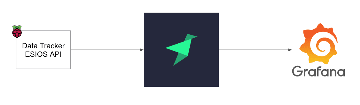
The infrastructure I used to automate the data tracker was a Raspberry Pi I have at home. So the code is continuously running and sending data into Tinybird. I have to say, though, that on some nights, the internet connection in my neighborhood goes down for a few minutes and breaks the execution, so it's not the best solution. Ideally, it should run on a host with a guaranteed connection. But anyways, I've added a backfill script that allows you to ingest data from the last 24 hours. Big problems, big solutions.
Design
From the ESIO API the idea is to bring data by indicator, and date range and the data returned by the ESIOS API has the following format:
{
  "indicator": {
    "name": "Composited indicator 2",
    "short_name": null,
    "id": 59526,
    "composited": true,
    "step_type": "linear",
    "disaggregated": false,
    "magnitud": null,
    "tiempo": [
      {
        "name": "Diez minutos",
        "id": 154
      }
    ],
    "geos": [
      {
        "geo_id": 1,
        "geo_name": "geo1"
      }
    ],
    "values_updated_at": "2015-09-15T08:34:34+02:00",
    "values_sum": 18,
    "values": [
      {
        "value": 4,
        "datetime": "2015-09-15T04:34:34.000+02:00",
        "datetime_utc": "2015-09-15T02:34:34Z",
        "geo_id": 1,
        "geo_name": "geo1"
      }
    ]
  }
}
It doesn't matter the indicator or the date range, the format will always be the same. This makes it easier to define a process in Tinybird: all the records will be saved, for simplicity, in a landing data source. Later, using materializations, different metrics will be saved in different materialized views to optimize the latency of the endpoints that will feed Grafana.
The landing data source (called landing_ds) has the following schema:
DESCRIPTION >
    Landing Electric Indicators

SCHEMA >
    `last_update` DateTime `json:$.last_update`,
    `datetime` DateTime `json:$.datetime`,
    `datetime_utc` DateTime `json:$.datetime_utc`,
    `tz_time` DateTime `json:$.tz_time`,
    `geo_id` UInt16 `json:$.geo_id`,
    `geo_name` String `json:$.geo_name`,
    `metric_id` UInt16 `json:$.metric_id`,
    `metric_name` String `json:$.metric_name`,
    `value` Float64  `json:$.value`

ENGINE "MergeTree"
ENGINE_SORTING_KEY "metric_id, last_update"
last_update is a DateTime parameter that indicates when the data was updated in Tinybird. For some metrics, data is updated in ESIOS every 5 minutes, others every 10 minutes, and so on. So the tracker runs every 5 minutes to bring in the most up to date data. The way records are ingested from the tracker into Tinybird is through the Events API, and that's why the JSON path of each column is included in the data source definition.
So now, the data flows from the ESIOS API into the landing_ds data source in Tinybird.
To create the materializations, the pipes read data from the landing data source and filter it using the metric_id field. That's why this field is part of the sorting key to make the process more efficient. Let me show you an example.
The following pipe (called generation.pipe) filters the electric generation records from landing_ds:
NODE materialize
DESCRIPTION >
    Filter records for generation metrics

SQL >

    SELECT
            last_update,
            datetime,
            datetime_utc,
            tz_time,
            geo_id,
            geo_name,
            metric_id,
            metric_name,
            value
        FROM landing_ds
    WHERE metric_id IN (2038, 2039, 2040, 2041, 2042, 2043, 2044, 2045, 2046, 2047, 2048, 2049, 2050, 2051)

TYPE materialized
DATASOURCE generation_mv
And the previous records are saved in the following data source called generation_mv.datasource
DESCRIPTION >
   Electric Generation Real-Time


SCHEMA >
   `last_update` DateTime,
   `datetime` DateTime,
   `datetime_utc` DateTime,
   `tz_time` DateTime,
   `geo_id` UInt16,
   `geo_name` String,
   `metric_id` UInt16,
   `metric_name` String,
   `value` Float64


ENGINE "ReplacingMergeTree"
ENGINE_SORTING_KEY "metric_id, metric_name, datetime"
ENGINE_PARTITION_KEY "toYYYYMM(datetime)"
ENGINE_VER "last_update"
The engine is a ReplacingMergeTree to guarantee the unicity of each record by metric_id, metric_name, and datetime. So only there will only be one metric for each datetime.
The next step is to prepare the endpoint to retrieve the values to show graphically from Grafana. So for this particular case, the endpoint is called generation_ep.pipe
NODE generation_node
DESCRIPTION >
    Generation timeseries

SQL >
    %
    SELECT
        toTimezone(datetime, 'Europe/Madrid') datetime,
        metric_name,
        value
    FROM generation_mv FINAL
    WHERE 1=1
        {\% if defined(start_datetime) %}
        AND toTimezone(datetime, 'Europe/Madrid') >= {{DateTime(start_datetime)}}
        {\% end %}
        {\% if defined(end_datetime) %}
        AND toTimezone(datetime, 'Europe/Madrid') <= {{DateTime(end_datetime)}}
        {\% end %}

TYPE ENDPOINT
Data visualization
Grafana is the tool choosen for this purpose and there are two options:
If you already have a Grafana instance, install the Infinity plugin and create a time series dashboard to monitor previous results.
In the Grafana folder of the project a
docker-compose.yamlfile exists that contains a Grafana instance that has installed the Infinity plugin. It creates the connection if you provide the Tinybird token and url and there is a dashboard that will be created once the Grafana image is up and where all the metrics calculated in this project are shown graphically. Also in the Docker Compose, there is a tool that will check every hour the dashboards and will export the .json file if they have been updated or created. This will allow us to have the dashboards saved securely in a git repository.
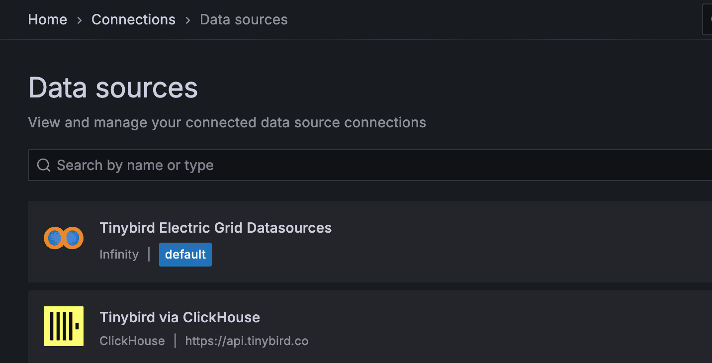
If you follow the second approach, after making Grafana to run, go to connections, and in the datasources section you should see a default Tinybird data source created using the Infinity plugin. Also, since now Tinybird can be connected directly to Grafana using the Clickhouse® plugin there is another extra connection created with that plugin called Tinybird via ClickHouse®.
Also In the dashboard section there should be a dashboard that shows electric KPIs.
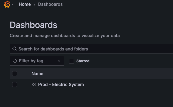
To be able to see all the graphs in that dashboard, you must create all the Tinybird resources. Otherwise, you'll see errors in some of them. And of course ingest data on them, otherwise they'll be blank.
Feel free to add more indicators to the dashboard and try how it works!
Take a look to the documentation of how to connect Grafana to Tinybird using the native connector.
Insights
While the data available from ESIOS doesn't reveal the exact cause of the blackout, it does provide valuable insights into how the Spanish electricity system operates, and maybe even some clues about what could have happened.
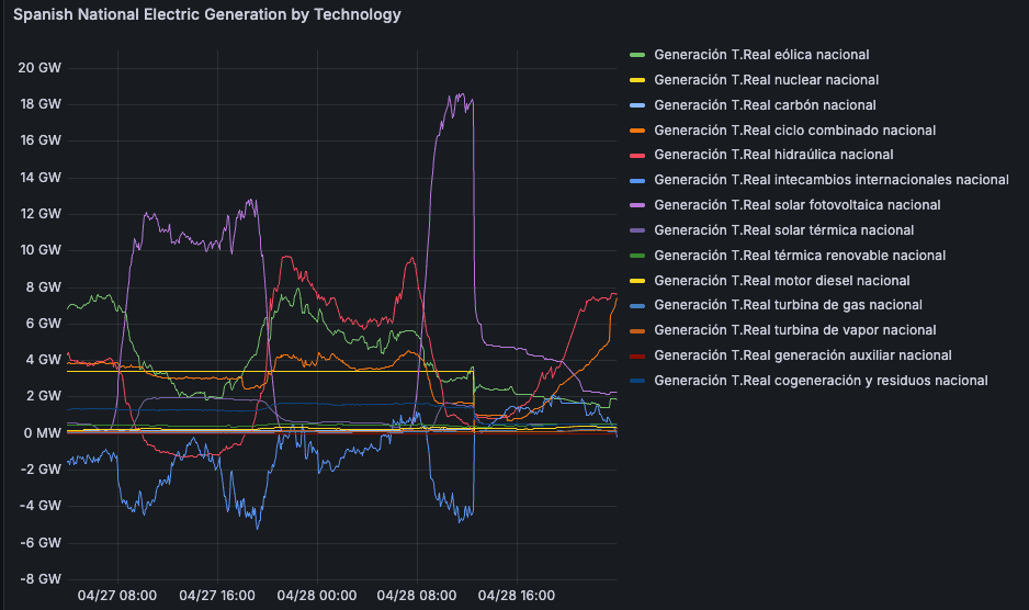
Spanish national electric generation by technology
Spain's electricity production is remarkably diverse, with at least 13 different generation technologies. Among them, nuclear, gas, hydro, wind, and solar power are the dominant sources. Spain also maintains strong international electricity exchanges with France, Portugal, Andorra, and Morocco, handling more than 8,500 MW. This variety makes Spain's electric system quite resilient from a supply security perspective.
During midday hours on sunny days, especially in summer, solar energy (purple line) covers a large portion of the electricity demand. Meanwhile, hydro (red line) and international exchanges (light blue line) often show negative values. That means Spain isn't just meeting its own electricity needs during those hours, it's exporting energy to its neighbors. In fact, Spain has been a net exporter of electricity since 2021. In other seasons, solar contributes less due to shorter daylight hours, but on sunny days it still dominates midday production, with wind energy playing a bigger role.
At night in summer, the main contributors shift to gas (orange line) and hydro. Wind often picks up at night as well, providing more than during the day, but of course, wind can't be controlled. This is crucial because electricity supply and demand must be balanced in real time: every megawatt generated must be consumed immediately to keep the grid stable.
Daily spot prices
All of this also explains electricity prices. Unsurprisingly, during midday in summer, when solar generation peaks, electricity prices drop to near zero. Free energy! (Well, not quite free, but definitely cheaper for everyone's electricity bill.)
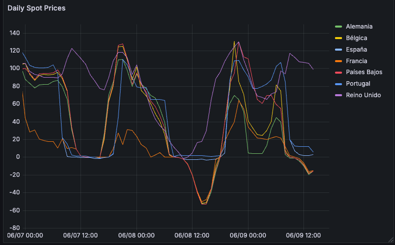
Spain and Portugal share the same electricity market, so their prices are typically very similar. However, after the blackout, electricity in Spain has been slightly cheaper than in Portugal. This could be because Spain is limiting exports to Portugal, likely as a precaution until the root cause of the blackout is fully understood.
The most expensive hours tend to be when demand peaks, early morning and evening, when solar isn't available and wind might not be strong enough. That's when gas steps in, and prices go up.
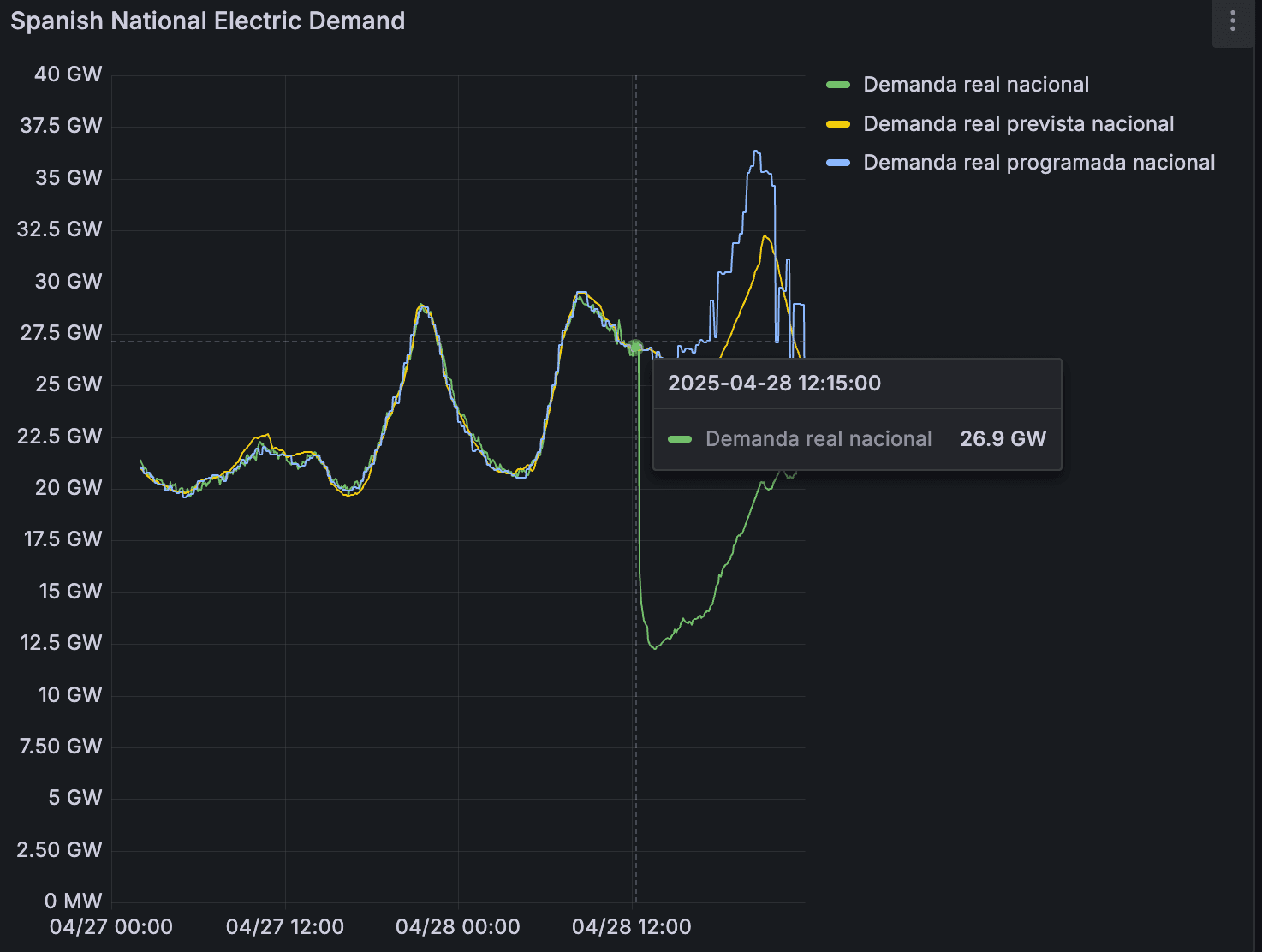
Spanish national electric demand
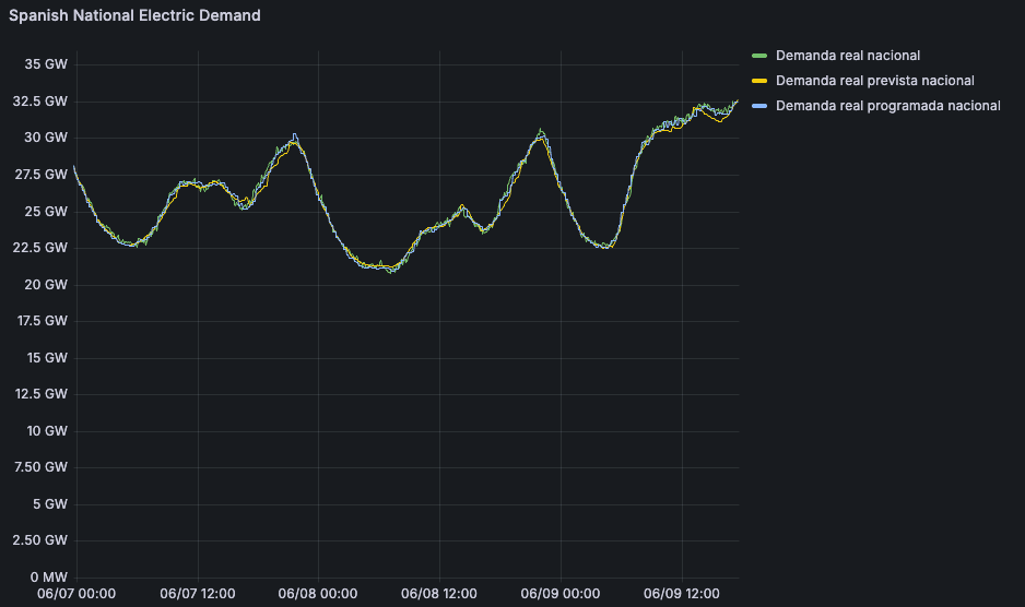
When comparing the day of the blackout to the day before and after, electricity generation patterns weren't dramatically different. Demand was slightly lower, probably due to the good weather at the time.
Nuclear was providing the same amount of energy that day as it does nowadays, but gas is now providing twice as much as it did on the day of the blackout. This is because demand was lower during those days, at 12:00, it was 27 GW, and now at the same time, it's over 31 GW.
Causes of the blackout
As for the cause of the blackout, honestly, no one knows for sure yet. But experts seem to agree on one thing: it likely wasn't just one issue, but a combination of at least two or more events that occurred within seconds. The data suggests one of these might have been a sudden drop in solar production. However, it doesn't look like generation capacity was the issue, today, for example, the grid handles nearly 20 GW of solar at peak hours, slightly more than the day of the blackout.
Another piece of the puzzle seems to be related to international exchanges. Those connections were abruptly cut off at the time of the blackout, leaving Spain unable to import power from neighboring countries just when it might have needed it most.
Conclusions
This doesn't rule out other problems, there were probably several, and it may be hard to predict exactly how to prevent a similar event in the future. But optimistically, maybe it was just such a rare chain of events that we won't see anything like it again in our lifetime.
Try it yourself
If you're curious about how real-time data can help make sense of critical infrastructure like the electrical grid, this project is a great starting point.
Deploy your own version:
curl https://tinybird.co | sh
tb login
tb local start
git clone git@github.com:ienva/ree_analytics_demo.git
cd ree_analytics_demo/tinybird
tb --cloud deploy
And use the Tinybird native Grafana connector to track KPIs, generate alerts, and experiment with new indicators.
Got ideas for more metrics or improvements? Open an issue or PR on GitHub. And if you build something cool, share it with us in our Slack community, we'd love to see what you're working on.