


When you’re trying to process huge amounts of data in real-time, there are some best practices to follow. These are hard-learned lessons from years of building real-time systems at huge scale. Now, we're sharing them with you.
The 5 Rules of Fast Queries
At Tinybird, we want our users to be able to go fast. Both when building queries, and then when those queries run. So, we've created a cheatsheet of rules you can consult whenever you need to go fast.
We like to call them The 5 Rules of Fast Queries:
- Rule № 1 ⟶ The best data is the data you don’t write.
- Rule № 2 ⟶ The second best data is the data you don’t read.
- Rule № 3 ⟶ Sequential reads are 100x faster.
- Rule № 4 ⟶ The less data you process (after read), the better.
- Rule № 5 ⟶ Move complex operations later in the processing pipeline.
Let’s go one by one, analyzing the performance improvement after the implementation of each rule using data stored in Tinybird. We will use the well-known NYC Taxi Trip dataset. You can get a sample here and import it directly into Tinybird by creating a new Data Source from your dashboard.
Rule 1: The best data is the data you don’t write
This rule seems obvious, but it’s not always followed. There is no reason to save data that you don’t need: it will impact the memory needed (and the money!) and the queries will take more time, so it only has disadvantages.
Rule 2: The second best data is the data you don’t read
To avoid reading data that you don’t need, you should apply filters as soon as possible.
Filtering is the fastest operation, so you should always filter first.
Using the NYC taxi data, let’s suppose we want a list of the trips whose distance is greater than 10 miles and that took place between ‘2017-01-31 14:00:00’ and ‘2017-01-31 15:00:00’. Additionally, we want to get those trips ordered by date.
Let’s see the difference in performance when we apply the filters at the end of our query execution versus the beginning.
First, let’s start the first approach by ordering all the data by date:
Once the data is sorted, we filter it:
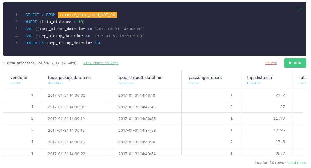
This first approach takes around 30-60 ms, if you add the processed time of both nodes.
Pay attention to the statistics: The first node scanned 139.26k rows processed 10.31 MB of data. The second node scanned 24.58k rows and 1.82 MB of data. Why would we scan 139.26k rows in the first place if we just really need to scan 24.58k?
It’s important to be aware that these two values directly impact the query execution time and also affect other queries you may be running at the same time. IO bandwidth is also something you need to keep in mind.
Now, let’s see what happens if the filter is applied before the sorting:
As you can see, if the filter is applied before the sorting, the query takes < 10 ms. If you take a look at the size of the data read, it’s 1.82MB, while the number of rows read is 24.58k. Compared to the previous approach, these are much smaller and more efficient.
This significant difference happens because in the first approach, we are sorting all the data available (even the data that we don’t need for our query) while in the second approach, we are sorting just the rows we need.
Filtering is the fastest operation, so always filter first.
Rule 3: Sequential reads are 100x faster
To be able to carry out sequential reads, it’s essential to define indexes correctly. These indexes should be defined based on the queries that we're going to perform. In this example, we'll simulate indexing data by sorting our tables before we query them to see how filtering by non-indexed columns affects performance.
Always index the columns by which you plan to filter. Sequential reads can be up to 100x faster when working with large amounts of data.
For example, if we want to query the data and filter by tpep_pickup_time, let’s compare what happens when the data is sorted by tpep_pickup_time versus when it’s sorted by any other column.
In the first approach, we will sort the data by another column, for instance, passenger_count:
Once we have the data sorted by passenger_count, we filter it by tpep_pickup_time:
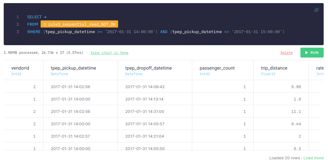
This approach takes around 5-10 ms, the number of scanned rows is 26.73k and the size of data is 1.98MB.
For the second approach, we'll sort the data by tpep_pickup_time:
And once it’s sorted by date, we filter it:
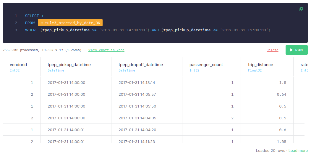
We can see that if the data is sorted by tpep_pickup_time and the query uses tpep_pickup_time for filtering, it just takes 1-2 ms, scans only 10.35k rows, and processes only 765.53 KB. The first approach, filtering by another column, takes around 5-10 ms, scans 26.73k rows, and processes 1.98 MB.
It’s important to highlight that the more data we have, the greater the difference between both approaches. When dealing with tons of data, sequential reads can be up 100x faster or more.
Therefore, it’s essential to define the indexes taking into account the queries that will be made.
Rule 4: The less data you process (after read), the better
The less data you process, the faster and cheaper your queries will be. So, if you just need two columns, only retrieve two columns in your SELECT.
Let’s suppose that for our use case, we just need three columns: vendorid, tpep_pickup_datetime, and trip_distance.
Don't run query operations over columns you don't need.
Let’s analyze the difference between selecting all the columns versus just the ones we need.
When we select all the columns, the query takes around 140-180 ms and processes 718.55 MB of data:
However, when we select just the columns we need, the query only takes around 35-60 ms and process ~20% of the data:
As we mentioned before, you can check how the size of scanned data is much less, now just 155.36MB. With analytical databases, if you do not need to retrieve a column, those files are not read and it is much more efficient.
Therefore, you should only process the data that you need.
Rule 5: Move complex operations later in the processing pipeline
Complex operations, such as joins or aggregations, should be performed as late as possible in the processing pipeline. This is because in the first steps you should filter all the data, so the number of rows at the end will be less than at the beginning and, therefore, the cost of executing complex operations will be lower.
So first, let’s aggregate the data:
Now, let’s apply the filter:
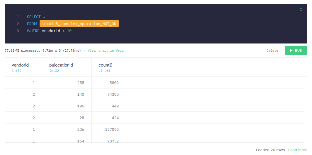
If the aggregations are performing before filtering, the query takes around 50-70 ms in total, and it scans 9.71 million rows and processes 77.68 MB.
In general, do SQL operations in this order: 1. Filter - 2. JOIN - 3. Aggregate.
Let’s see what happens if we filter first and then aggregate:
This approach takes only 20-40 ms even though the number of scanned rows and the size of data is the same as in the previous approach.
Therefore, you should perform complex operations as late as possible in the processing pipeline.
Some additional guidance
In addition to these 5 rules, here’s some more general advice for optimal queries in Tinybird:
Avoid Full Scans
The less data you read in your queries, the faster they are. There are different strategies you can follow in Tinybird to avoid reading all the data in a data source (doing a full scan) from your queries:
- Always filter first
- Use indices by setting a proper
ENGINE_SORTING_KEYin the Data Source. - The column names present in the
ENGINE_SORTING_KEYshould be the ones you will use for filtering in theWHEREclause. You don’t need to sort by all the columns you use for filtering, only the ones to filter first. - The order of the columns in the
ENGINE_SORTING_KEYis important: from left to right ordered by relevance (the more important ones for filtering) and cardinality (less cardinality goes first).
Avoid Big Joins
When doing a JOIN in Tinybird, the data in the right Data Source is loaded in memory to perform the JOIN. Therefore, it’s recommended to avoid joining big Data Sources by filtering the data in the right Data Source.
JOINs over tables of more than 1M rows might lead to MEMORY_LIMIT errors when used in Materialized Views, affecting ingestion.
A common pattern to improve JOIN performance is the one below:
New to Tinybird?
Tinybird is a real-time data platform for developers and data teams. Ingest data from anywhere, query it with SQL, and publish your (optimized) queries as low-latency APIs in a click. You can sign up for free with no time limit and no credit card required.