



One thing that surprised me after working with dozens of data teams from different companies to help them scale their analytical pipelines is that some mistakes repeat continuously. Almost every performance issue looks different on the surface, but they normally have the same root cause. The problem is not that ClickHouse®, our backend database, works badly. It is that we treat it as a transactional database.
Normally, data teams land on Tinybird looking for a better tool for their analytical use cases, but the first solution they build follows the same transactional database approach. Same queries. Same data model.
OLTP (Online Transaction Processing) databases are made to handle lots of inserts and small reads. OLAP (Online Analytical Processing) databases are made to handle complex reads across millions of rows as fast as possible. Common use cases are dashboards, BI, and time series analysis.
Here are seven mistakes I see repeatedly, how I normally identify them, and the effect the fixes had on one production workload.
Rule 1: Just read the data you need to show
One of the most common mistakes I have seen is not filtering the data correctly. The query reads and scans millions of rows to finally return a couple of dozen data points. That is one of the first things I normally check: how many rows and bytes are read, and how many are returned?
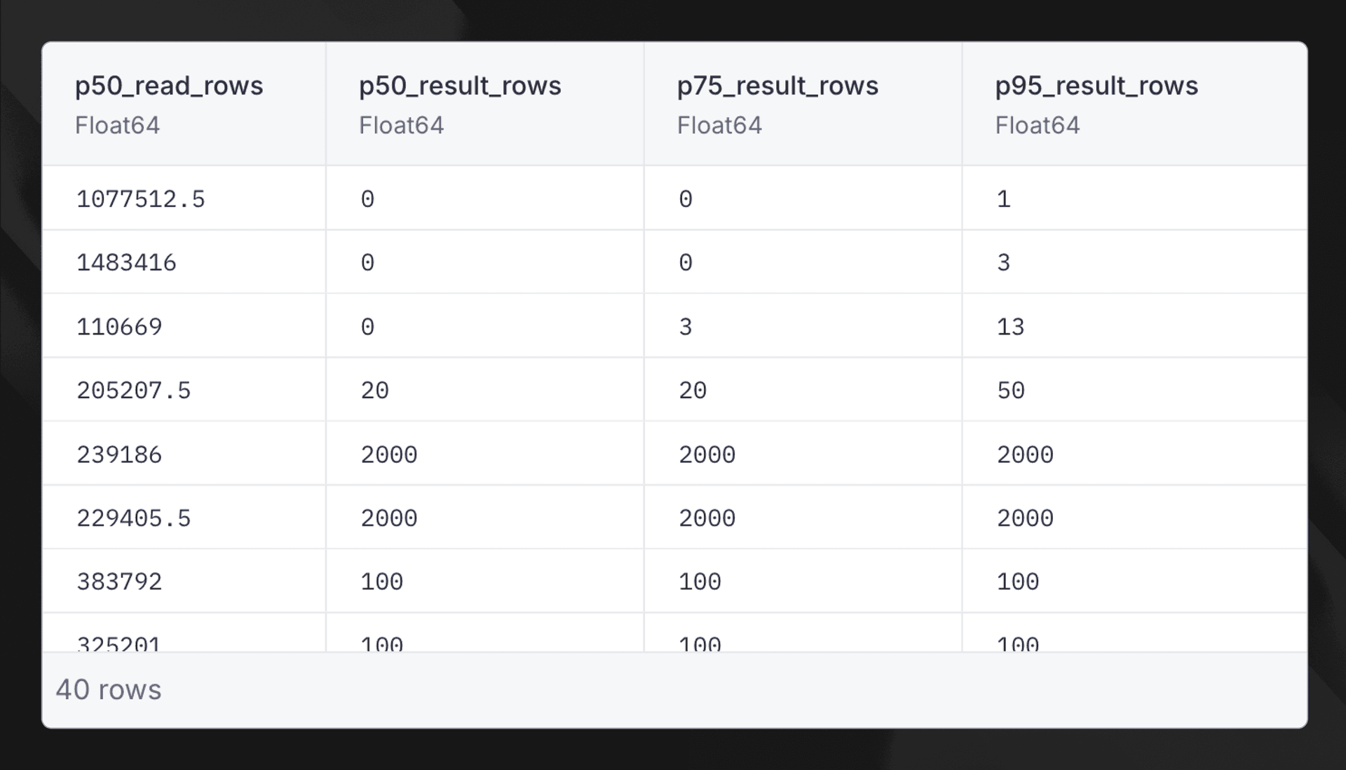
If a query reads millions of rows to return no values and consumes a lot of resources, something is not correctly defined. My first recommendation is always to filter the data as early as possible. It prevents the query from spending memory and CPU on data that is not needed for the final result.
The examples use two source data files. table_a contains users:
# table_a.datasource

SCHEMA >
    `user_id` String `json:$.user_id`,
    `user_name` String `json:$.user_name`,
    `is_active` UInt8 `json:$.is_active`

ENGINE "MergeTree"
ENGINE_SORTING_KEY "user_id"
table_b contains addresses. Its initial sorting key supports lookups by user_id, but not country filters:
# table_b.datasource

SCHEMA >
    `user_id` String `json:$.user_id`,
    `address` String `json:$.address`,
    `country` String `json:$.country`,
    `updated_at` DateTime `json:$.updated_at`

ENGINE "MergeTree"
ENGINE_SORTING_KEY "user_id"
DESCRIPTION >
    table_a - table_b join endpoint

NODE result
SQL >
    %
    SELECT
        a.user_id,
        a.user_name,
        b.address,
        b.country
    FROM table_a AS a
    INNER JOIN table_b AS b
        ON a.user_id = b.user_id
    WHERE a.is_active = 1
    {\% if defined(country_value) %}
        AND upper(b.country) = upper({{ String(country_value) }})
    {\% end %}

TYPE endpoint
In this example, the filters appear after the join. Depending on the query plan, ClickHouse can push some predicates down automatically. I prefer to make the filtered inputs explicit and then check the result with EXPLAIN. That makes the intended execution order clear and confirms whether less data actually reaches the join.
I would write the endpoint like this:
DESCRIPTION >
    table_a - table_b join endpoint

NODE table_a_filtered
SQL >
    SELECT
        user_id,
        user_name
    FROM table_a
    WHERE is_active = 1

NODE table_b_filtered
SQL >
    %
    SELECT
        user_id,
        address,
        country
    FROM table_b
    {\% if defined(country_value) %}
        WHERE upper(country) = upper({{ String(country_value) }})
    {\% end %}

NODE result
SQL >
    SELECT
        a.user_id,
        a.user_name,
        b.address,
        b.country
    FROM table_a_filtered AS a
    INNER JOIN table_b_filtered AS b
        ON a.user_id = b.user_id

TYPE endpoint
The SELECT * is gone because ClickHouse is a columnar database. Selecting only the columns we need reduces the volume of data read. The filters are also explicit before the join. Still, a different query shape is not automatically faster. I use EXPLAIN indexes = 1 and the query statistics to check whether it really reduces rows, granules, or bytes read.
Rule 2: Take advantage of sorting keys
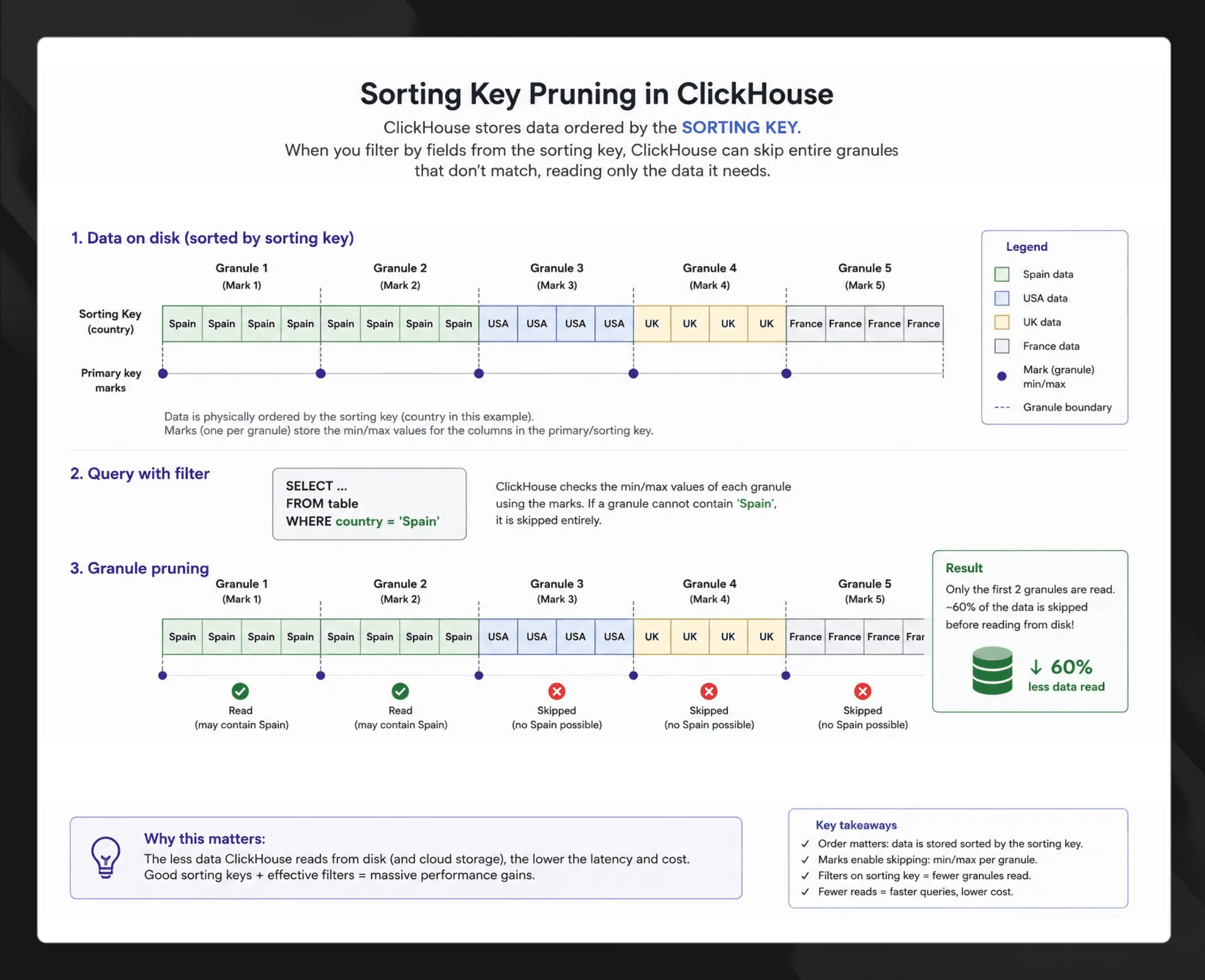
Sorting keys define how data is ordered on disk. Using them in filters allows ClickHouse's sparse primary index to skip granules, which can reduce latency and resource usage.
I normally define sorting keys from the final query patterns. In this example, country is a candidate for the sorting key of table_b if most requests filter by country. Its position depends on the other common filters and their selectivity. Again, EXPLAIN indexes = 1, read_rows, and read_bytes tell us whether the key is helping.
There is one important detail here: the current upper(country) predicate cannot use a sorting key on the raw country value for range pruning. Once Rule 3 normalizes the country during ingestion, the endpoint can filter the stored value directly. If the workload normally filters by country before joining on user_id, the key could be:
ENGINE "MergeTree"
ENGINE_SORTING_KEY "country, user_id"
Rule 3: Reduce operations at query time
Another recurring mistake I have seen is performing the same transformation every time a query runs when it can be done once during ingestion. For example:
WHERE toDate(timestamp) = today()
Or:
WHERE upper(country) = 'SPAIN'
If the date or normalized country is used in many queries, we can calculate it once during ingestion. For the country example, we can use a materialized view. Tinybird applies the Pipe to each inserted block and stores the result in a target data source:
# clean_data_mv.pipe

NODE transform
SQL >
    SELECT
        address,
        user_id,
        upper(country) AS country
    FROM table_b

TYPE MATERIALIZED
DATASOURCE table_b_transform
This is the data source where the transformed rows are stored:
# table_b_transform.datasource
SCHEMA >
    `address` String,
    `user_id` String,
    `country` String

ENGINE "MergeTree"
ENGINE_SORTING_KEY "country, user_id"
And the endpoint can now filter the precomputed value directly:
NODE table_a_filtered
SQL >
    SELECT
        user_id,
        user_name
    FROM table_a
    WHERE is_active = 1

NODE table_b_filtered
SQL >
    %
    SELECT
        address,
        user_id,
        country
    FROM table_b_transform
    {\% if defined(country_value) %}
        WHERE country = upper({{ String(country_value) }})
    {\% end %}

NODE result
SQL >
    SELECT
        a.user_id,
        a.user_name,
        b.address,
        b.country
    FROM table_a_filtered AS a
    INNER JOIN table_b_filtered AS b
        ON a.user_id = b.user_id

TYPE endpoint
This moves work from query time to ingestion time. It also uses ingestion CPU and additional storage, so it makes sense when the same transformation is read much more often than it is written. As with the previous changes, measure both sides before materializing it.
Rule 4: Define data types properly
As in the previous rules, defining the data model correctly can reduce the bytes processed and therefore the cost. But the goal is not to choose the smallest type blindly. I choose the narrowest type that represents the data correctly and then verify the effect with sample data and production query statistics.
These are my main recommendations for data types:
- Use
Nullablewhen null has meaning. A nullable column stores an additional null mask and can limit some optimizations. Avoid it when a non-null default accurately represents the domain, but do not replace meaningful nulls just to save space. - Use
LowCardinality(String)for repeated string values. Dimensions such as country, status, or event type often benefit from dictionary encoding. The benefit depends on the number and distribution of distinct values, so treat thresholds such as 10,000 values as a starting point, not a rule. - Use
FixedString(N)only for values that are exactlyNbytes. A fixed-length identifier does not automatically perform better asFixedString. Prefer native types such asUUIDwhen they fit, and benchmark againstStringwhen they do not. - Choose
DecimalorFloatbased on correctness first. UseDecimalwhen exact decimal arithmetic matters, such as money. Use floating-point types only when approximation is acceptable. - Choose integer width and sign together.
UInt32andInt32both use 32 bits.UInt32represents a larger non-negative range, whileInt32represents negative values. Pick the smallest width that covers the required range. - Store only the time precision you query. Use
Datefor calendar dates,DateTimefor second precision, andDateTime64only when sub-second precision is required.
# table_b_transform.datasource
SCHEMA >
    `address` String,
    `user_id` String,
    `country` LowCardinality(String)

ENGINE "MergeTree"
ENGINE_SORTING_KEY "country, user_id"
This is the same target data source from Rule 3, now using LowCardinality(String) for country.
Rule 5: Joins are costly
That joins are costly does not mean they cannot be used. Sometimes they are necessary at query time. The important thing is to reduce the rows and bytes on both sides before joining them. Filter each input first, select only the required columns, and aggregate before the join when that does not change the result. I also keep the join-key types compatible to avoid casts and larger hash tables.
I do not move a join later just because it is a join. I use EXPLAIN and query statistics to check which ordering keeps the same result while processing less data.
Rule 6: Avoid calculating the same thing several times
This mistake normally comes from not understanding how materialized views work in ClickHouse. They can calculate shared transformations and aggregations once for each inserted block instead of once per API request.
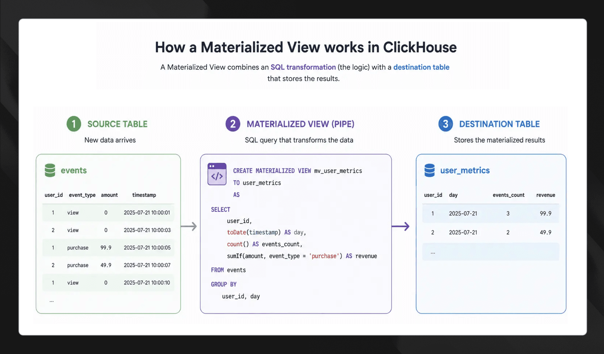
One of the most difficult things to understand about materialized views in ClickHouse and Tinybird is that they are based on two resources:
- A materialization Pipe containing the SQL transformation.
- A target data source storing the Pipe output.
When a block is inserted into the origin data source, Tinybird runs that block through the materialization Pipe and inserts the result into the target. The complexity moves from the endpoint to ingestion, where each inserted block is processed once. This improves read performance when the result is reused often enough to justify the extra ingestion CPU and storage.
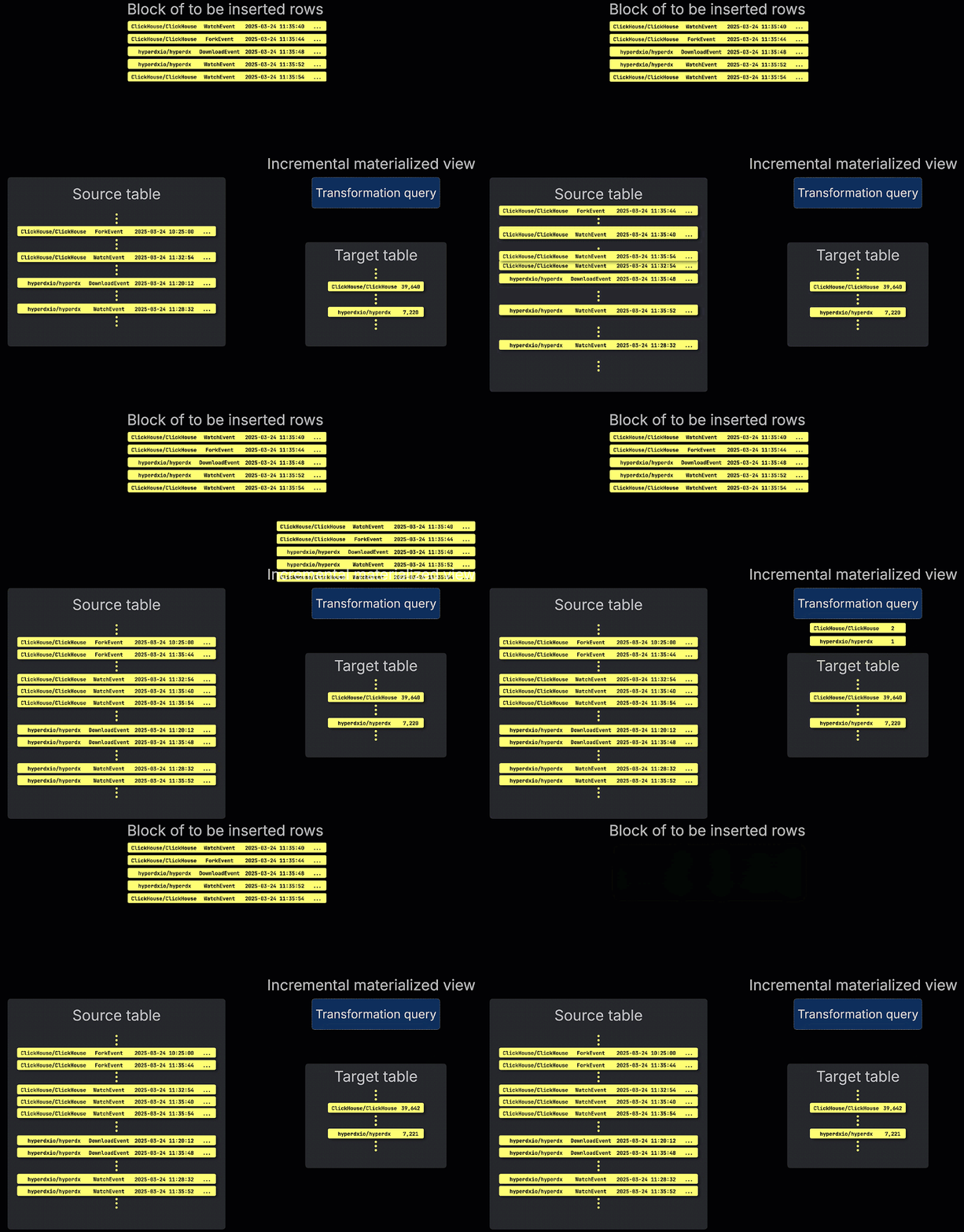
This also adds some limitations. How do we remove duplicates if they are not in the same inserted block? What happens with aggregations? ClickHouse has engines that combine partial results over time, although that combination can still require work at query time.
ReplacingMergeTree
ReplacingMergeTree is useful for removing duplicates. It removes rows with the same sorting key during background merges and, with a version column, keeps the row with the highest version.
The disadvantage is that background merges are asynchronous. A normal query can return more than one version before the relevant parts have merged. When the query must return the deduplicated result immediately, use FINAL:
# user_addresses.datasource

SCHEMA >
    `user_id` String,
    `address` String,
    `country` LowCardinality(String),
    `updated_at` DateTime

ENGINE "ReplacingMergeTree"
ENGINE_SORTING_KEY "user_id"
ENGINE_VER "updated_at"
SELECT
    user_id,
    address,
    country
FROM user_addresses FINAL
WHERE user_id = 'user-123'
FINAL applies the replacement logic while the query runs. It does not physically merge the stored parts, and it adds overhead. I only use it when that consistency requirement justifies the cost.
AggregatingMergeTree
AggregatingMergeTree stores intermediate aggregate states grouped by the sorting key. The materialization Pipe has to write a -State value:
NODE aggregate_latest_address
SQL >
    SELECT
        user_id,
        argMaxState(address, updated_at) AS latest_address
    FROM table_b
    GROUP BY user_id

TYPE MATERIALIZED
DATASOURCE latest_user_address
The target schema also has to declare the complete aggregate type, including its argument types:
SCHEMA >
    `user_id` String,
    `latest_address` AggregateFunction(argMax, String, DateTime)

ENGINE "AggregatingMergeTree"
ENGINE_SORTING_KEY "user_id"
Then the endpoint applies the matching -Merge combinator and groups by the sorting key:
NODE result
SQL >
    SELECT
        user_id,
        argMaxMerge(latest_address) AS latest_address
    FROM latest_user_address
    GROUP BY user_id

TYPE endpoint
SummingMergeTree
SummingMergeTree is similar, but it is intended for additive metrics. It combines numeric columns by the sorting key during background merges. Queries must still aggregate rows when unmerged parts can contain the same key.
Joins in materialized views
A final important detail about joins: a materialized view is triggered only by inserts into the leftmost data source in FROM. The right side of a join is read when a left-side block arrives. Inserts into the right-side data source do not update rows that were already materialized.
The right side can also be scanned in full for every inserted block. To avoid that, restrict it to the keys from the current left-side block:
DESCRIPTION >
    table_a - table_b join endpoint

NODE table_a_filtered
SQL >
    SELECT
        user_id,
        user_name
    FROM table_a
    WHERE is_active = 1

NODE table_b_filtered
SQL >
    SELECT
        user_id,
        address,
        country
    FROM table_b_transform
    WHERE user_id IN (SELECT user_id FROM table_a_filtered)

NODE result
SQL >
    SELECT
        a.user_id,
        a.user_name,
        b.address,
        b.country
    FROM table_a_filtered AS a
    INNER JOIN table_b_filtered AS b
        ON a.user_id = b.user_id

TYPE MATERIALIZED
DATASOURCE active_user_addresses
The target data source stores the materialized rows:
# active_user_addresses.datasource

SCHEMA >
    `user_id` String,
    `user_name` String,
    `address` String,
    `country` String

ENGINE "MergeTree"
ENGINE_SORTING_KEY "country, user_id"
This limits the right-side rows passed into the join to keys in the inserted block. To reduce the physical scan as well, the layout has to support user_id lookups with a compatible sorting key, projection, or separate lookup data source. For time-bounded or ASOF joins, I also add an explicit time range. None of this changes the trigger behavior: right-side updates still do not recalculate old materialized output.
I see this error a lot: materialization Pipes consuming more than 10 CPU seconds and gigabytes of memory for only a few megabytes of inserted data. You can monitor them in the tinybird.datasources_ops_log service data source, where cpu_time is reported in seconds and memory_usage in bytes.
Rule 7: Define partition keys carefully
Another common error that is sometimes missed during optimization is the partition key. Partitioning is mainly a data-management tool. It groups rows into independent parts so ClickHouse can drop, move, or apply TTLs to complete partitions. It can also reduce reads when a query filters on the partition expression, but the sorting key remains the main tool for skipping data inside a partition.
I only define a partition key when it matches how the data is queried or managed. Too many partitions create too many small parts and add overhead to inserts, background merges, and some reads. As a general rule, a few large partitions are better than thousands of very small ones.
How to identify optimization opportunities
One of the most useful tools for optimizing SQL queries is EXPLAIN. EXPLAIN indexes = 1 shows whether the sorting key is pruning parts and granules. Other variants show the query plan and the operations ClickHouse performs at each stage.
I compare that plan with runtime data from system.query_log, ProfileEvents, or Tinybird service data sources. The questions are simple: is the query reading more rows and bytes than expected? Is it allocating too much memory? Is it repeating work that could be done once?
For selective filters, PREWHERE can read the filter columns first and load the remaining columns only for matching rows. ClickHouse often moves suitable WHERE conditions there automatically, so I only use it explicitly after measuring the query and confirming the read pattern.
How to monitor in Tinybird
This section is an extra for anyone who wants to monitor endpoint and ingestion consumption in Tinybird. The service data sources expose this telemetry as queryable data. For API endpoints and Query API requests, I normally use tinybird.pipe_stats_rt and check:
duration: request duration in seconds.cpu_time: CPU time in seconds.memory_usage: query memory consumption in bytes.read_rowsandread_bytes: rows and bytes scanned.result_rows: rows returned.
The time series view is also useful for seeing changes in these metrics after a deployment. If performance gets worse after changing a resource, it is normally visible there. Just make sure to compare equivalent time windows and account for traffic changes before attributing the result to the query.
Tinybird also provides an organization metrics template that exposes metrics in Prometheus format. From there, you can visualize them in Grafana and create alerts for errors or resource thresholds.
Some numbers
The following charts come from a real optimization process for a small startup. Its workload was using roughly three times the capacity it needed, and the cost had become a problem. The charts show per-request CPU-time quantiles in seconds from tinybird.pipe_stats_rt. To validate this kind of result, I also compare the request volume and workload mix across the before and after windows.
| Metric | Before | After | Change |
|---|---|---|---|
| Endpoint p95 CPU time | About 5 seconds | Below 1 second | More than 80% lower |
| Query API p99 CPU time | About 12 seconds | About 4 to 6 seconds | About 50 to 67% lower |
| Required instance capacity | Baseline | One third of baseline | 3x smaller |
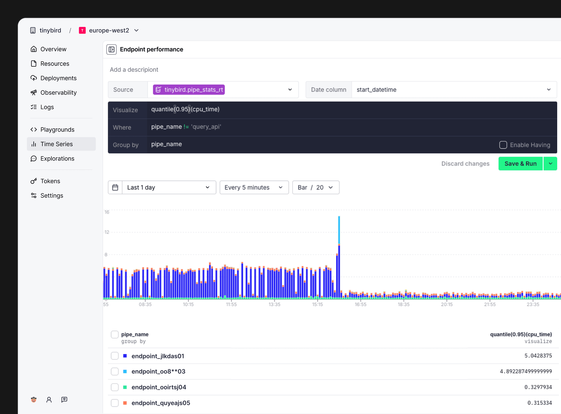
The endpoint chart excludes query_api and groups requests by Pipe. After applying most of the recommendations in this post, p95 per-request CPU time fell from roughly five seconds to below one second.
The customer also used the Query API to run arbitrary SQL. This case is more difficult to optimize because every request can execute a different query. We started by finding the query shapes that ran most often and consumed the most resources.
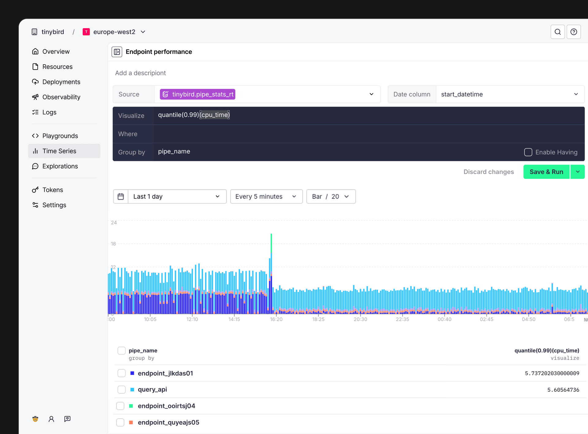
The most frequent queries were missing some filters. We fixed those and moved the stable request shapes to API endpoints, where the SQL could be reviewed and tested. Query API p99 CPU time fell from roughly 12 seconds to between 4 and 6 seconds.
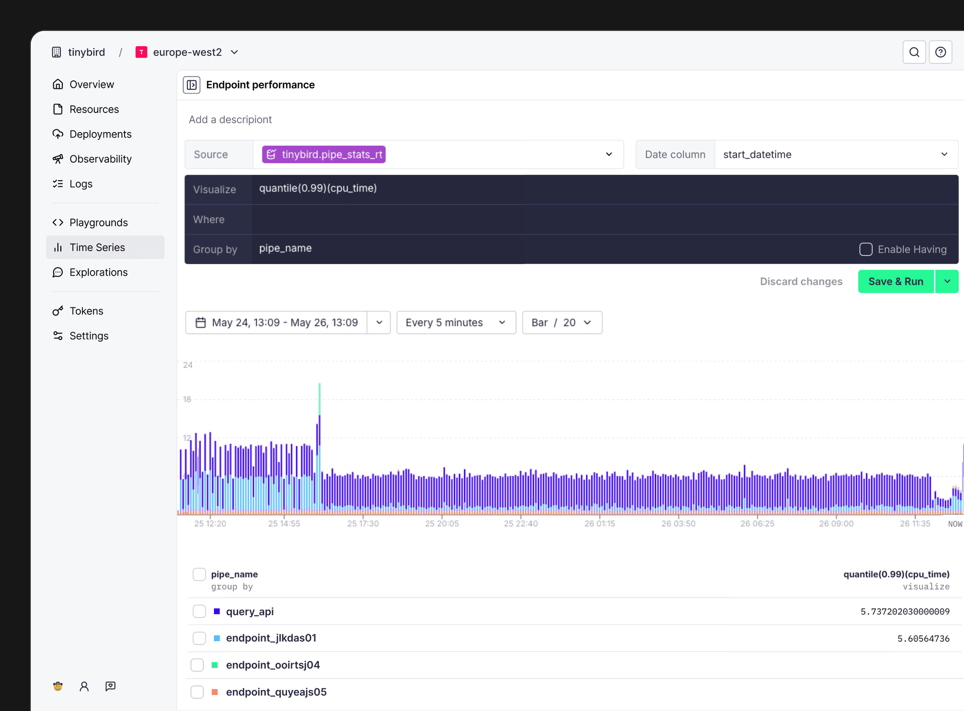
Together, these changes allowed the customer to run the workload on an instance with one third of the previous capacity. The exact cost reduction depends on the infrastructure and pricing model, so capacity is the useful comparison here.
Make ClickHouse do less work
Every optimization in ClickHouse is ultimately about the same thing: making the engine do less work. Read less data, move less data, calculate less data, and avoid repeating expensive calculations.
I normally start with EXPLAIN, query logs, and Tinybird service data sources. I measure rows, bytes, CPU, memory, and latency, change one part of the query or schema, and measure again. The goal is not to apply every rule in this post. It is to find where the workload is doing unnecessary work and remove it.